What Is R2 in Statistics: A Clear Guide for 2026

R² is the proportion of variation in the outcome your model explains, written on a 0 to 1 scale, where 0.70 means the model captures 70% of the variance. It's a useful first read on fit, but it can still mislead you if you stop there.

You've probably seen the number appear right after fitting a regression line, then wondered whether it means the model is useful or just mathematically tidy. That's the right instinct, because R² tells you something real, but not everything that matters.

Table of Contents

• Why R² Matters in Everyday Regression Work
• The Intuition Behind Explained and Unexplained Variation
• The R² Formula and What Each Piece Means
• A Worked Example You Can Calculate by Hand
• Adjusted R² and When It Beats Plain R²
• Common Misreadings That Trip People Up
• Putting R² in Context for Model Evaluation

Why R² Matters in Everyday Regression Work

You fit a regression, the dashboard flashes 0.74, and suddenly everyone wants a verdict. That is why R² gets so much attention in statistics, business analytics, and machine learning, because it gives a quick read on how much of the outcome your model is accounting for.

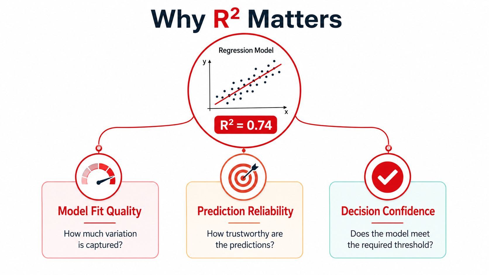
A useful mental model is straightforward. R² answers a narrow question, how much of the variation in the thing you want to predict does the model explain? That is why it is commonly treated as a goodness-of-fit measure in regression work, and why it shows up early in model review. The standard interpretation uses a 0 to 1 scale, so a value like 0.70 is read as the model explaining 70% of the variance in the outcome, with the remaining variation still outside the model's reach. The core definition and range are summarized in the coefficient of determination on Wikipedia the coefficient of determination on Wikipedia, and the same basic interpretation is laid out in a statistical note on regression interpretation from the University of Auckland.

The first question R² answers

Students often get tripped up because they expect R² to answer every question at once. It does not. It answers one question well, which is whether the model captures a meaningful share of the variation in the response.

Practical rule: treat R² as a fit summary, not a final verdict.

That is why the number matters in everyday work. It helps you compare models, decide whether a regression is even worth discussing, and get a first read on whether the signal is strong or weak. It cannot tell you whether the relationship is causal, whether the residuals are behaving, or whether the model will generalize cleanly to new data. Those gaps are exactly where confusion starts, and exactly why the rest of the guide has to go beyond the single decimal.

The Intuition Behind Explained and Unexplained Variation

A classroom-grade analogy works better than a formula at first. Suppose students' test scores vary quite a bit, and a teacher wants to know how much of that spread can be linked to study hours. Some of the difference in scores lines up with study time, and some of it comes from everything else, like prior knowledge, sleep, stress, and plain randomness.

Three pieces are hiding inside the spread

That spread has three parts in regression language. There is the total variation, which is the full amount of scatter in the observed outcome. There is the explained variation, which is the part your model accounts for. And there is the residual variation, which is what remains after the model makes its predictions.

R² is the share of total variation that falls into the explained category. If the model explains most of the spread, R² moves toward 1. If the model explains almost none of it, R² sits near 0. That basic decomposition of total variation into explained and unexplained parts is the backbone of the statistic, and it is why statisticians treat it as more than a decorative output number.

The easiest trap here is to treat the unexplained part as failure. It is not. In real data, leftover variation is normal, and often expected. A good model does not eliminate all noise, it explains enough of the pattern to be useful for the task you care about.

A model can still be valuable even when it leaves plenty of variation behind. The question is whether the remaining noise still matters for your decision.

That intuition matters because it keeps you from asking R² to do work it was never designed to do. The statistic is about proportion, not perfection. Once you see that split between explained and unexplained variation, the formula starts to feel like shorthand rather than a trick.

The R² Formula and What Each Piece Means

A student looking at R² for the first time often sees a neat fraction and assumes the whole story is hidden in the algebra. The formula is short, but each symbol is doing a lot of work. R² = 1 - RSS/TSS means the model is being judged by how much variation it leaves behind compared with the total variation in the outcome.

What RSS and TSS mean in plain language

RSS means residual sum of squares. It is the sum of the squared prediction errors, so it measures how far the model's predictions are from the observed values overall. A larger RSS means the model is missing more of the pattern.

TSS means total sum of squares. It measures the total spread of the observed values around their average, before the model gets involved. In other words, TSS is the amount of variation sitting on the table before any prediction starts.

The formula uses 1 - RSS/TSS because it starts with the whole amount of variation and subtracts the part the model fails to explain. If the residual part is small relative to the total, the explained part is large. That is the logic behind the statistic in the regression framework.

The usual teaching interpretation is straightforward. If RSS is tiny compared with TSS, then R² is close to 1, which means the fitted line or curve tracks the observed data closely. If RSS is almost as large as TSS, then R² is close to 0, which means the model is barely doing better than a simple baseline.

Why people meet it through correlation first

In simple linear regression, R² is also the square of the correlation coefficient. That is why students often meet it first as “the square of r,” not as a full variance decomposition. The two views fit together, but the variance view holds up better once you move beyond one predictor.

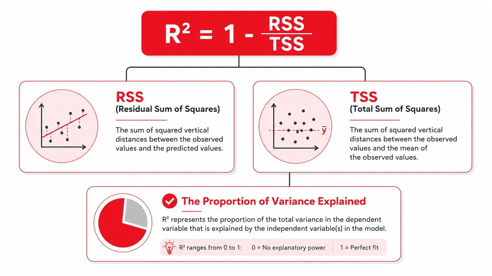
The best way to read the formula is as a ledger. The model starts with total variation, leaves some of it in the residuals, and the rest is the share it explains. That is the whole statistic in one line.

A Worked Example You Can Calculate by Hand

A small table is the fastest way to make R² feel real. Suppose you're looking at a toy dataset with five rows, and a regression model gives you predicted values for each observed x. The numbers below are chosen to make the arithmetic easy to follow on paper.

Add the squared residuals and you get RSS = 1.10. That's the total amount of error the model leaves behind after predicting all five points. The residuals are small for four rows and a little larger for one row, which is why the total stays modest.

Now find the average of the observed y values. The mean is 4.8. Subtract that mean from each observed value, square the differences, and add them up to get TSS = 23.2. This is the full spread of the outcome before the model explains anything.

Turning the arithmetic into R²

Now use the formula:

R² = 1 - RSS/TSS = 1 - 1.10/23.2

That gives R² = 0.9526, which you'd usually round to 0.95. In plain English, the model explains about 95% of the variance in the outcome on this tiny dataset.

The decimal only looks abstract until you compare it with the raw spread in the data. Then it becomes obvious why a model with small residuals earns a high R².

A few students get tripped up here because they expect R² to come directly from the predictions alone. It doesn't. You need both the prediction errors and the total spread around the mean, because R² is a comparison against the baseline variation in the data.

That comparison is the lesson. A model with a low RSS relative to TSS is doing useful work. A model with a high RSS relative to TSS isn't capturing much structure at all.

Adjusted R² and When It Beats Plain R²

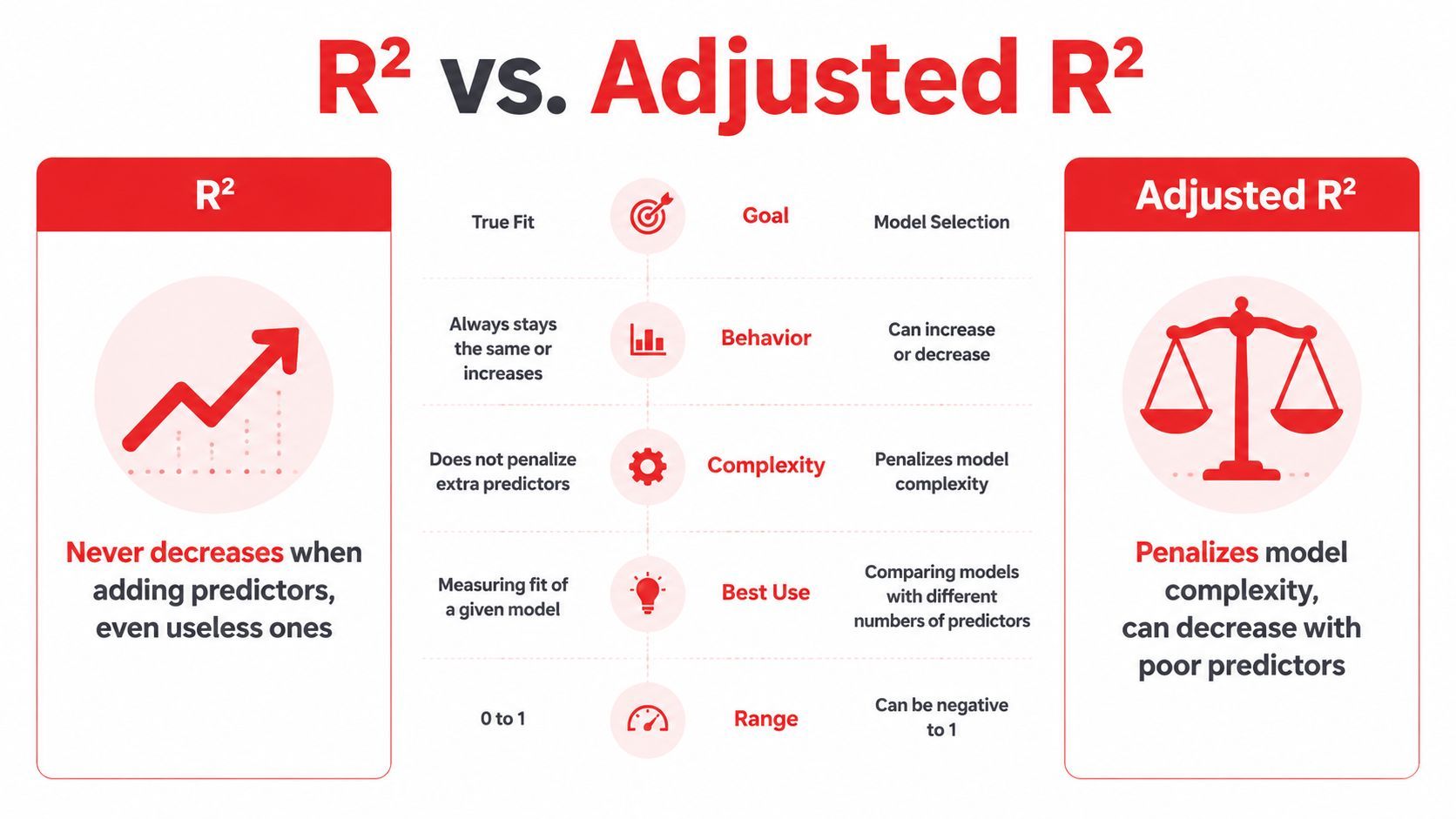
Plain R² has a built-in weakness, it never goes down when you add more predictors. Even a useless extra variable can make the fit look a little better on the training data, which is why R² can reward complexity that doesn't earn its keep.

Why adjusted R² exists

Adjusted R² fixes that problem by penalizing extra predictors. Instead of asking only how much variation the model explains, it also asks whether each added variable is paying for its own complexity. If a new predictor doesn't improve the model enough, adjusted R² can stay flat or drop.

That's why adjusted R² is often the better number for model selection. If you're comparing several regression models with different numbers of predictors, plain R² will almost always favor the more complicated one. Adjusted R² is more cautious, which is useful when feature lists get long and some inputs are probably just noise.

When each one belongs in the report

Use plain R² when you want to describe fit in a simple, familiar way. Use adjusted R² when you're choosing among competing multiple regression models and need to know whether the extra predictors are really worth it.

Here's the cleanest rule of thumb.

• Use R² when the audience wants a direct read on how much variation the model captures.
• Use adjusted R² when you're comparing models with different numbers of predictors.
• Treat a rising R² with caution if the added variables don't have a clear reason to be there.

In practice, the two numbers often travel together. The plain version tells you the raw fit, and the adjusted version tells you whether that fit still looks convincing after complexity is counted. If the numbers disagree, that disagreement is useful, because it usually means one of your predictors is contributing less than it looks like on the surface.

Common Misreadings That Trip People Up

The biggest mistake is thinking a high R² proves the model is right. It doesn't. A strong fit can coexist with a weak causal story, especially when the model is describing association rather than mechanism.

High R² is not the same as causation

A high R² only says the model explains a lot of variation in the observed data. It does not tell you why that variation exists, and it definitely does not prove that one variable caused another. If the wrong conclusion matters, you need a design or identification strategy that goes beyond regression fit.

Low R² is not automatic failure

A low R² can still be acceptable when the outcome is noisy or when your goal is directional prediction rather than tight reconstruction. Students often panic when they see a small value, but context matters. In fields where the signal is faint, a modest share of explained variance can still be practically useful.

R² can miss nonlinear structure

R² is tied to the fit of the model you gave it. If the true relationship bends, curves, or changes shape in a way your linear model can't capture, a disappointing R² may be warning you about model form rather than about the absence of structure. That's why residual plots matter, they can reveal patterns that a single fit statistic hides.

Don't compare it blindly across very different settings

Two R² values from different outcomes are not always directly comparable. A model for one target can naturally produce a very different range of fit than a model for another target, because the outcomes behave differently. The number is meaningful inside its own context first.

Time series need extra caution

With time-dependent data, a tempting R² can hide serial patterns in the residuals. A model may look decent on paper while still leaving structure in the errors that violates the assumptions behind the regression. If the data move over time, residual inspection matters even more.

Diagnostic habit: when a fit number looks attractive, ask what the residuals are doing before you trust the headline.

The safest reflex is to treat R² as one clue among several. It can tell you whether the model captures a meaningful share of variation, but it can also flatter a bad model, especially if you don't inspect what's left behind.

Putting R² in Context for Model Evaluation

A good regression review doesn't stop at R². It places the number next to adjusted R², residual plots, prediction error on held-out data, and domain knowledge about whether the explained variation is enough to matter in the decision.

If you want a simple checklist, use this order after fitting a model.

• Check R² and adjusted R². Look at fit and complexity together, not separately.
• Inspect residual plots. Look for curvature, clusters, or time-based patterns.
• Evaluate prediction error on held-out data. A model that fits the sample well can still disappoint on new data.
• Ask whether the explained variation is meaningful. A statistically neat model isn't automatically useful if the uncovered variation still drives the decision.

That last question is the one people skip most often. If the use case is pricing, planning, forecasting, or risk review, the important issue is not whether the number looks respectable. It's whether the model changes what you would do next.

The opening question was never just “what is R2 in statistics.” It was really, “Can I trust this regression output?” The answer is yes, if you read R² as a fit summary, check the residuals, and stop treating a single decimal as the full story. If you want a fast way to turn that discipline into a production workflow for AI-powered analytics or model review, start a project with Supagen.